Prava funkcija v programu VBA Excel
Desna funkcija je enaka kot pri funkciji delovnega lista in VBA, uporaba te funkcije je, da nam daje podniz iz določenega niza, vendar iskanje poteka od desne proti levi od niza, to je vrsta funkcije niza v VBA uporablja se s funkcijsko metodo application.worksheet.
DESNA funkcija v Excelu VBA, ki se uporablja za pridobivanje znakov na desni strani priloženih besedilnih vrednosti. V Excelu imamo veliko besedilnih funkcij za obdelavo podatkov, ki temeljijo na besedilu. Nekatere uporabne funkcije so LEN, LEFT, RIGHT, MID funkcija za pridobivanje znakov iz besedilnih vrednosti. Pogost primer uporabe teh funkcij je ločevanje imena in priimka ločeno od polnega imena.
Formula PRAVO je tudi na delovnem listu. V VBA se moramo za dostop do funkcije VBA RIGHT zanašati na razred funkcije delovnega lista, namesto tega pa imamo vgrajeno funkcijo RIGHT tudi v VBA.
Zdaj pa si oglejte spodnjo sintakso formule VBA RIGHT.
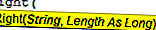
- Niz: To je naša vrednost in iz te vrednosti poskušamo izvleči znake z desne strani niza.
- Dolžina: Koliko znakov potrebujemo iz priloženega niza . Če potrebujemo štiri znake z desne strani, lahko argument navedemo kot 4.
Če je na primer niz »Mobilni telefon« in če želimo izvleči samo besedo »Telefon«, lahko navedemo argument, kot je prikazan spodaj.
DESNO (»Mobilni telefon«, 5)
Razlog, zakaj sem omenil 5, ker ima beseda "Telefon" 5 črk. V naslednjem oddelku članka bomo videli, kako ga lahko uporabimo v VBA.
Primeri funkcije Excel VBA Right
Sledijo primeri pravilne funkcije VBA Excel.
To predlogo programa VBA Right Function Excel lahko prenesete tukaj - Predloga programa VBA Right Function Excel
Primer # 1
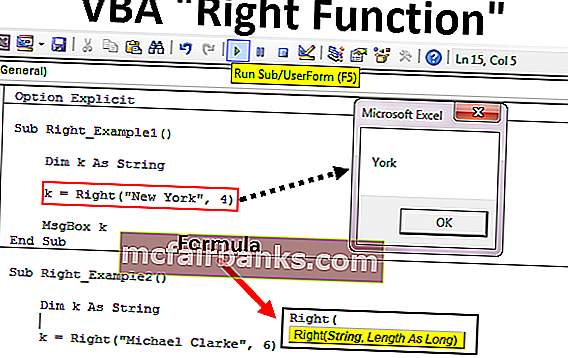
Pokazal vam bom preprost primer za začetek postopka. Predpostavimo, da imate niz »New York«, in če želite izvleči 3 znake z desne strani, sledite spodnjim korakom za pisanje kode.
1. korak: Spremenljivko prijavite kot niz VBA.
Koda:
Sub Right_Example1 () Dim k As String End Sub
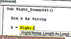
2. korak: Zdaj bomo tej spremenljivki vrednost dodelili z uporabo funkcije DESNO.
Koda:
Sub Right_Example1 () Dim k As String k = Right (End Sub
3. korak: Prvi argument je String, naš niz za ta primer pa je "New York".
Koda:
Sub Right_Example1 () Dim k As String k = Right ("New York", End Sub 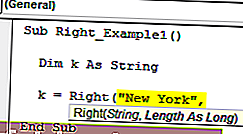
Korak 4: Naslednje je, koliko znakov potrebujemo iz priloženega niza. V tem primeru potrebujemo 3 znake.
Koda:
Sub Right_Example1 () Dim k As String k = Right ("New York", 3) End Sub 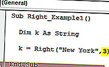
5. korak: Imamo dva argumenta, zato smo končali. Zdaj dodelite vrednost tej spremenljivki v polju za sporočila v VBA.
Koda:
Sub Right_Example1 () Dim k As String k = Right ("New York", 3) MsgBox k End Sub 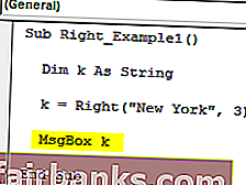
Zaženite kodo s tipko F5 ali ročno in si oglejte rezultat v oknu za sporočila.
V desni strani besede "New York" so 3 znaki "ork".
Zdaj bom dolžino spremenil s 3 na 4, da dobim polno vrednost.
Koda:
Sub Right_Example1 () Dim k As String k = Right ("New York", 4) MsgBox k End Sub 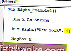
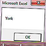
Zaženite to kodo ročno ali s tipko F5, dobili bomo "York".
2. primer
Zdaj pa si oglejte še en primer, tokrat upoštevajte vrednost niza kot "Michael Clarke".
Če navedete dolžino 6, bomo kot rezultat dobili "Clarke".
Koda:
Sub Right_Example1 () Dim k As String k = Right ("Michael Clarke", 6) MsgBox k End Sub 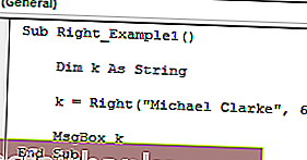
Zaženite to kodo s tipko F5 ali ročno, da vidite rezultat.
Dinamična desna funkcija v Excelu VBA
Če upoštevate prejšnja dva primera, smo ročno podali številke argumentov dolžine. Toda to ni pravi postopek za opravljanje dela.
In each of the string right-side characters are different in each case. We cannot refer to the length of the characters manually for each value differently. This where the other string function “Instr” plays a vital role.
Instr function returns the supplied character position in the supplied string value. For example, Instr (1,” Bangalore”,”a”) return the position of the letter “a” in the string “Bangalore” from the first (1) character.
In this case, the result is 2 because from the first character position of the letter “a” is the 2nd position.
If I change the starting position from 1 to 3 it will return 5.
Instr (3,” Bangalore”,”a”).
The reason why it returns 5 because I mentioned the starting position to look for the letter “a” only from the 3rd letter. So the position of the second appeared “a” is 5.
So, to find the space character of the of each string we can use this. Once we find the space character position we need to minus that from a total length of the string by using LEN.
For example in the string “New York” the total number of characters is 8 including space, and the position of the space character is 4th. So 8-4 = 4 right will extract 4 characters from the right.
Now, look at the below code for your reference.
Code:
Sub Right_Example3() Dim k As String Dim L As String Dim S As String L = Len("Michael Clarke") S = InStr(1, "Michael Clarke", " ") k = Right("Michael Clarke", L - S) MsgBox k End Sub 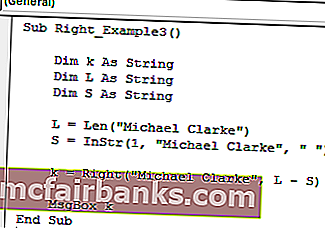
In the above code variable “L” will return 14 and variable “S” will return 8.
In the VBA right formula, I have applied L – S i.e. 14-8 = 6. So from right side 6 characters i.e. “Clarke”.
Loops with Right Function in Excel VBA
When we need to apply the VBA RIGHT function with many cells we need to include this inside the loops. For example, look at the below image.
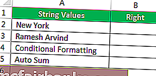
We cannot apply many lines of the code to extract a string from the right side. So we need to include loops. The below code will do it for the above data.
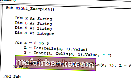
Code:
Sub Right_Example4() Dim k As String Dim L As String Dim S As String Dim a As Integer For a = 2 To 5 L = Len(Cells(a, 1).Value) S = InStr(1, Cells(a, 1).Value, " ") Cells(a, 2).Value = Right(Cells(a, 1), L - S) Next a End Sub
The result of this code is as follows.